Histopathologic Cancer Detection

Cancer is the name given to a Collection of Related Diseases. In all types of Cancer’s, some of the Body’s cells Begin to Divide Without Stopping and Spread into Surrounding Tissues.

When a surgeon operates to remove a Primary Cancer, one or more of the nearby (regional) Lymph Nodes may be removed as well. Removal of one lymph node is called a Biopsy. When many lymph nodes are removed, it’s called Lymph Node Sampling or Lymph Node Dissection. When cancer has spread to Lymph Nodes i.e known as Metastasis, then there’s a Higher Risk that the Cancer might come back after Surgery. The tissue that’s removed is looked at under the microscope by a Pathologist for the Presence of Cancer Cells.

Lymph Nodes 

Lymph vessels route lymph fluid through nodes throughout the body. Lymph nodes are small structures that work as filters for harmful substances. They contain immune cells that can help fight infection by attacking and destroying germs that are carried in through the lymph fluid.

Metastasis 

Metastasis is the Spread of Cancer Cells to new areas of the body, often by way of the lymph system or bloodstream. A metastatic cancer, or metastatic tumor, is one that has spread from the primary site of origin, or where it started, into different areas of the body.

Histopathology

Histology is the study of Tissues, and Pathology is the Study of Disease. So, taken together, Histopathology literally means the Study of Tissues as relates to Disease. A histopathology report describes the tissue that has been sent for examination and the features of what the cancer looks like under the microscope. A histopathology report is sometimes called a Biopsy Report or a pathology report.

Digital Pathological Scans

Digital pathology is a sub-field of pathology that focuses on data management based on information generated from Digitized Specimen Slides. Through the use of computer-based technology, digital pathology utilizes virtual microscopy. Glass slides are converted into digital slides that can be viewed, managed, shared and analyzed on a computer monitor. With the practice of Whole-Slide Imaging (WSI), which is another name for virtual microscopy, the field of digital pathology is growing and has applications in diagnostic medicine, with the goal of achieving efficient and cheaper diagnoses, prognosis, and prediction of diseases.

So, the task here is to Detect the presence of Metastases (Tumor Tissue) in Pathological Scans Using Neural Networks with Best Possible Accuracy.

Objectives and Constraints

    • No Low Latency Constraints.

    • Predictions have to be Very Accurate.

    • The False Negative Values should be as low as Possible.

Performance Metrics

    • AUC
    • F1 Score
    • Recall Score

Data

The Data here is from the Histopathological Scans. A positive label indicates that the center 32×32 px region of a patch contains at least one pixel of Tumor Tissue. Tumor tissue in the outer region of the patch does not influence the label. This outer region is provided to enable fully-convolutional models that do not use zero-padding, to ensure consistent behaviour when applied to a Whole Slide Image(WSI).

  • This Dataset was prepared on PCam (Patch Camelyon) which was prepared on Camelyon16 Data.
  • It is Smaller version of Camelyon16 Data.
  • The Original PCam dataset contains duplicate images due to its Probabilistic Sampling, however, the version presented on Kaggle does not contain duplicates.

The Data can be downloaded from https://www.kaggle.com/c/histopathologic-cancer-detection/data

Files

    • Train : 5.87 GB
    • Test : 1.53 GB
    • Train_Labels: 9.02 MB

Train and Test Data consists only Images. Let’s visualize some images Randomly.

  •  

The above shown images are randomly selected from the entire data set. The tissues with presence of cancer cells are represented with red patches and the tissues without cancer cells are represented with green patches. With a normal eye, it is very difficult, otherwise impossible to classify directly by seeing the images.  May be not that tough for the trained eye i.e. Pathologist. 

Cleaning the Data

As, the inputs here are Images, let’s check the images that are very bright and dark. As, this sort of images do not contain any information, we can drop them. This can be achieved by using the code snippet shown below.

Splitting the Data

The Data has to be split down into Train and Validation Data, so that the model can be trained on the Train Data and the evaluation of the model can be done on the Validation Data. Here we are splitting the data randomly in the ratio 90:10 i.e. 90% as Train Data and 10% as Validation Data.

Building Input Data Pipeline using tf.data

In the traditional methods, most of the processing is done by CPU, Heavy Lifting is done by the GPU and both CPU and GPU have to wait till the next batch is fed. Thus, this makes these methods Inefficient One!

To overcome this Tensorflow provides tf.data API to build the Efficient and Scalable Input Pipelines. This could be the somewhat painful process for the first time, but the most efficient pipelines can be built using Tensorflow’s Dataset Module i.e.  tf.data.  This API from Tensorflow allows us to build Highly Optimized Pipelines both for text and image data, using the resources from GPU efficiently by feeding the Data continuously by dividing it into batches. 

Let us understand tf.data by mapping it to the ETL Process i.e. Extract Transform and Load.
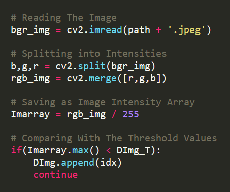
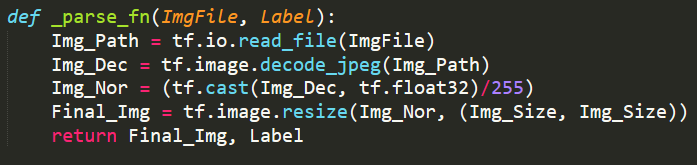
Extract Stage:

It is the phase of reading the data from a network storage or the local disk. In our case it is the Local Storage. So, the first step in this Pipeline is to create the dataset from the slices of File Names or Path’s.

Transform Stage:

Stage where the data is transformed from one form to other i.e. may be specific transformations related to the problem or the generic transformations. i.e. shown below

_parse_fn, here does the following things

    • Read the content of the specified file i.e. image.
    • Decodes the image.
    • Normalizes and Resizes the Image.

The snippet for the _parse_fn is shown below

The map function from python implements the above transformations for the sliced data. Then using the batch function, the sliced data is divided into the mini batches.

Load Stage:

In this phase the transformed data is loaded to the Accelerator i.e. CPU and GPU. In tf.data API we have pipelining option, i.e. this parallelizes the CPU and GPU processes by prefetching the next batch data as the current batch is under process. The code snippet for this is shown below.

Building the Model using Keras Sub Classing:

Two models were built using custom sub-classing code, one is just a simple Convolutional Neural network based Model and other if Transfer Learning based Model. Transfer Learning based model has performed well. The architecture for the transfer Learning based model is shown below. 

With Custom Keras Model Sub Classing, we can define exactly the pattern of operations in each layer including gradients. The code snippet for the above model using Keras Model Sub Classing is shown below

Training Model using tf.GradientTape

The above model is trained using tf.GradientTape API for automatic differentiation i.e. computing the gradient of the computation with respect to the inputs. Automatic Differentiation are set of techniques that can automatically compute the derivative of a function by repeatedly applying the Chain Rule. It is the fast and efficient method to compute gradients i.e. partial derivatives. So, to implement the  GradientTape we need to define 2 steps i.e.

    • Loss Function
    • Optimizer

The loss function here considered is Binary Cross Entropy and the Optimizer considered is Adam Optimizer.

The code snippet for implementing tf.GradientTape is shown below

The above model is trained with different tuning values for several epochs on data obtained from both tf.data Input Data Pipeline and Augmented Images mapped to the tf.data i.e with different augmentations like random_flip, adjusting saturation, adjusting brightness etc. The trained models are check-pointed using tf.train.CheckPoint API and saved using tf.saved_model API. The best model is obtained by Dropout rate =0.5, Learning rate of the Optimizer =0.001 and training the model for 10 Epochs. The Plots for the best model are shown below.

AUC Plot:

Accuracy Plot:

Loss Plot:

Testing the Model Performance

The performance of the above trained best model is tested on the test dataset containing 57,458 Images. AUC Score Obtained on these data by the best model is 97.77%.

The Preview of  Deployment Model Prototype using Flask is shown below.

Conclusions:

    • The Data given here is Images.
    • 32*32 Px has the actual Target Cells.
    • The first step done is Reading the Data.
    • Observed the Distribution of the Data.
    • Outlier’s or the Erroneous/ Less Information Points are Dropped Down.
    • Now, the Data is Split down in 90:10 Ratio.
    • These Images are read using the tf.data API.
    • Two Models were built on top of it.
    • These models are trained using GradientTape.
    • Checkpointing, and saving the models is performed using tf.train.Checkpoint and tf.saved_model.
    • Transfer Learning Based Model has performed better than the simple CNN Model.
    • The Best Model from these Models is selected and the prediction of the Test Data points is performed.
    • Kaggle Leader Board Score Obtained is Public : 97.34, Private : 97.77.
    • 1157 teams have been participated in this Competition, and score obtained is in the Top 7.6% of the Leader Board.


Thank you for Reading..!

While some of the code snippets are included in the blog, and for the full code you can check out this Jupyter Notebook on GitHub.

Useful Links and References:

  • https://en.wikipedia.org/wiki/Cancer
  • https://www.cancer.net/navigating-cancer-care/cancer-basics/what-metastasis
  • https://www.cancer.gov/about-cancer/understanding/what-is-cancer
  • https://en.wikipedia.org/wiki/Digital_pathology
  • https://www.webmd.com/cancer/cancer-pathology-results#1
  • https://www.verywellhealth.com/histopathology-2252152
  • https://www.cancer.org/cancer/cancer-basics/lymph-nodes-and-cancer.html
  • https://www.tensorflow.org/api_docs/python/tf/GradientTape
  • https://www.youtube.com/watch?v=T8AW0fKP0Hs
  • https://www.cs.toronto.edu/~rgrosse/courses/csc321_2018/slides/lec10.pdf
  • https://en.wikipedia.org/wiki/Automatic_differentiation
  • https://www.pyimagesearch.com/2020/03/23/using-tensorflow-and-gradienttape-to-train-a-keras-model/
  • https://www.kite.com/python/docs/tensorflow.GradientTape

Kranthi Kumar Valaboju